Attractor Networks, (A bit of) Computational Neuroscience Part III

Brains are comprised of networks of neurons connected by synapses, and these networks have greater computational properties than the neurons and synapses themselves. In this post, I am going to talk about a class of neural networks which I think are fascinating: attractor networks. These are recurrent neural networks with attractor states; these states and the dynamics governing an attractor networks evolution between attractor states endow these networks with powerful computational properties. Some attractor networks are useful models of neural circuits. It would be helpful to have a little knowledge of neuroscience and dynamical systems — fortunately for you my previous posts cover those topics: for an introduction to dynamical systems, you can read Part I, for an introduction to synapses, you can read Part II. You can probably get by without it though.

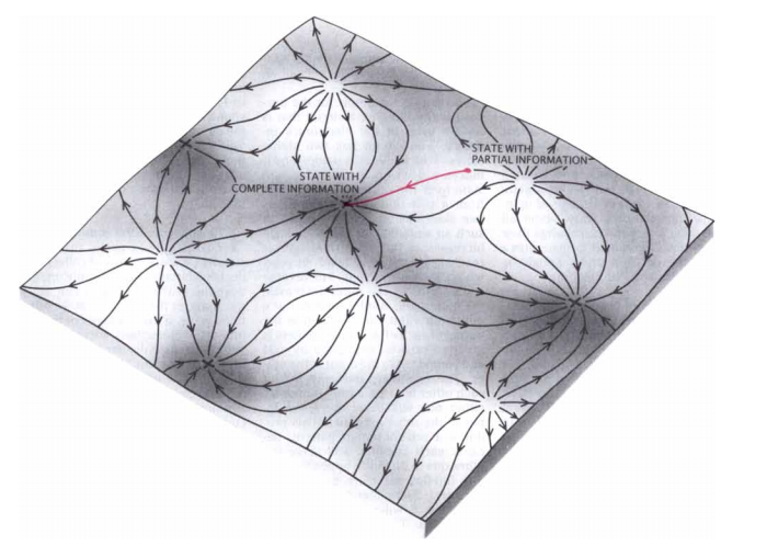
Attractor networks give rise to many interesting computational properties, e.g. categorization, filtering noise, integration, memorization [6]. These networks can shed light on the following questions. How can networks act stably and persistently? If we assume different neurons hold different pieces of information, how do neurons integrate this information? Furthermore, how can networks retrieve memories?

Through the lens of dynamical systems theory, these networks are easier to understand and thus the questions above can be answered more easily. Dynamical systems theory provides us with two levels of description:

• network space: The full state of the neural network, which is quite large and unwieldy.
• attractor space: A reduced space of the full neural network. Only includes points on the attractors.

Let’s look at two examples of attractor networks. The first we will look at is the Hopfield network, an artificial neural network. The second we will look at is a spiking neural network from [3] (Wang 2002).

Hopfield Network

Hopfield networks [2] (Hopfield 1982 ) are recurrent neural networks using binary neuron. Although not a spiking network model, its . It is a model of associative memory.

Through the lens of dynamical systems, learning is achieved by adjusting the network so that the to-be-learned patterns become attractors states, i.e. if the .

Network

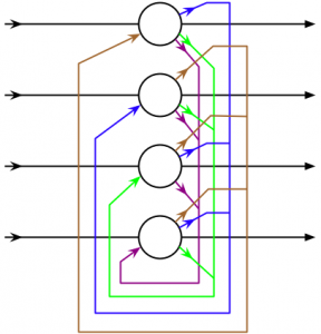
A Hopfield network is comprised of $N$ neurons $\vec{V}$ with thresholds $\theta$ (typically all identical and $=0$) and connections $W$. The topology of the network connections is simple: each neuron is connected to all other neurons except itself and all connections are symetric, or

$$\begin{align}w_{ij} &= 0 \text{ if } i=j \\w_{ij} &= w_{ji} \end{align}$$

The neurons $V$ in a Hopfield network have two states: on or off, i.e. $v_i \in \{-1, 1\}$.

Each state in a network is associated with an Energy. By updating the network, according to a rule below, the Energy decreases to a local minimum.

$$E = \frac{1}{2} \sum\limits_{i}\sum\limits_{j} w_{ij}V_{i}V_{j} – \sum\limits_{i}V_i\theta$$

remember	trash	pattern

The main parts of the code is below. You can find the full hopfield/tensor code here.

/**
* Step toward a fixed point in the Hopfield Network
* by reducing the energy in the Hopfield Network
* @param {HopfieldNetwork} network
*/
function update(network) {
    // V = 1 if WV > θ else -1
    const W = network.W,
    V = network.V,
    θ = network.θ;
    network.V = where(greaterEqual(dot(W, V),θ), 1, -1);
    return network;
}

    /**
     * Learn to store the patterns.
     * Set patterns as fixed points
     * using a Hebbian Learning scheme
     *
     * @param {Tensor} (M x N), i.e. M patterns or length N 
     * @param {HopfieldNetwork} network 
     * @returns {Tensor} (N x N) W a weight matrix
     */
    function learnHebbian(patterns, network) {
        let [M, N] = patterns.shape;
        let W = fillT([N, N], 0);
        for (let i=0; i < M; i++) {
            let pattern = patterns.get([i, ':']);
            W = W.add(outer(pattern, pattern));
        }
        // normalize
        network.W = W.div(M);
        // set trace = 0
        for (let i=0; i < N; i++) {
            network.W.set([i,i], 0);
        }
        return network;
    }

Dynamics

The dynamics, i.e. the update rule, of a Hopfield network as follows. If the state of neuron $i$ at time $t$ is $V_i^t$, then at time $t+1$, the state of that neuron is:

$$V_i^{t+1} = sign(\sum\limits_{j}W_{ij} \cdotp V_i)$$

where $\cdotp$ is the dot product and the $sign$ operator is what you can guess:

$sign(x) =\begin{cases}
1 &\text{ if } x \ge \theta,\\
-1 &\text{otherwise}
\end{cases}$

This should be pretty familiar if you have worked with artificial neural networks (for you computer scientists) or rate-networks (for you theoretical neuroscientists): its a thresholded linear combination of input activations and synaptic weights.

Learning Rule

To store a pattern, $V$, in a Hopfield network, the pattern must become a fixed point attractor, i.e. $V = update(\langle V, W \rangle)$. By setting the values of the weight matrix according the Hebbian Learning rule, the patterns become minimum energy states. The Hebbian Learning rule is not the only learning rule (see: Storkey Learning Rule).

Now, let’s prove that the Hebbian Learning rule results in fixed points:

claim : The Hebbian learning rule sets patterns as fixed points.

proof :

Let’s assume $V$ is a pattern stored in a Hopfield network such that $W_{ij} \propto V_iV_j$. We can now show $V$ is a fixed point by direct proof:

$$\begin{align} \vec{V} &= update(\langle \vec{V}, W \rangle)  & \text{ definition of fixed point } \\ V_i &= sign(\sum\limits_j W_{ij}V_j) & \text{update rule} \\V_i &= sign(\sum\limits_j V_i V_j V_j) & \text{Hebbian learning rule, i.e. } W_{ij}=V_iV_j \\V_i &= sign(\sum\limits_j V_i * 1) & \text{no matter the value of } V_j \text{ it will be 1} \\V_i &= sign(N * V_i) & \text{summing} \\V_i &= V_i & \text{N*V_i} \\ \hfill\blacksquare \end{align}$$

Spiking Attractors

Spiking attractor networks are fascinating: they suggest how brains are able to (1) act stably, (2) integrate information distributed across neurons, (3) recover memories etc. despite being composed of billions of seemingly cacophonous neurons. Lets consider a binary decision task in which a network receives two noisy signals: $A$ and $B$ and must choose which signal is stronger. Given the constraints of neural circuits, this is actually, quite a feat. If each neuron in each population receives a different Poisson spike train generated from its respective noisy signal, then each neuron within a population will possess different and potentially conflicting information about the state of the world. In order to perform the binary decision task, the network must be able to integrate information about both signals, which is distributed across many neurons and across time, and compare them. Additionally, in order for a selective population of neurons one selective population of neurons must drive the neural circuit and turn off competing coalitions of neurons.

Slow Reverberations

Below is an (approximate) implementation of [3] (X-J Wang 2002). This recurrent spiking network has 4 populations of neurons:

• (#0-#399) a population of inhibitory inter-neurons.
• (#400-1519) a population of background excitatory neurons which help sustain activity.
• (#1520-#1999) 2 selective populations, i.e. each receives input corresponding to a stimulus.

Essentially, the two selective populations recurrently stimulate themselves and inhibit each other through the inter-neurons. That is, they compete against each-other to drive the neural circuit. The reverberations (or the ramping up) of recurrent NMDA allows the network to integrate (or accumulate) information over time and across neurons to make a decision.

Here the network level is the membrane potential of each of the 2000 neurons and the activation of the synapses between each pair of neurons. The attractor level is the firing rates of two populations — a reduction of several orders of magnitude.

The default input to the model below is such that the network should make random decisions. Both selective populations receive spike trains of $40 hz$.

Above is a video of the simulation below, in case your computer runs this code slowly or if you are on mobile.

References

• [1] Tank, David W., and John J. Hopfield. “Collective computation in neuronlike circuits.” Scientific American 257.6 (1987): 104-115.
• [2] Hopfield, John J. “Neural networks and physical systems with emergent collective computational abilities.” Proceedings of the national academy of sciences 79.8 (1982): 2554-2558.
• [3] Wang, Xiao-Jing. “Probabilistic decision making by slow reverberation in cortical circuits.” Neuron 36.5 (2002): 955-968.
• [4] Wang, X. J. “Attractor network models.” Encyclopedia of neuroscience. Elsevier Ltd, 2010.
• [5] Dayan, Peter, and Laurence F. Abbott. Theoretical neuroscience. Vol. 806. Cambridge, MA: MIT Press, 2001.
• [6] Chris Eliasmith (2007) Attractor network. Scholarpedia, 2(10):1380.