
Synapses are the couplings between neurons, allowing signals to pass from one neuron to another. However, synapses are much more than mere relays: they play an important role in neural computation. The ongoing dramas of excitation and inhibition and of synaptic potentiation and depression give rise to your abilities to make decisions, learn, and remember. It’s amazing, really: collections of these microscopic junctions in your head can represent all sorts of things — your pet’s name, the layout of the New York subway system, how to ride a bike…
In this post, I give a rough overview of synapses: what they are, how they function, and how to model them. Specifically I will focus on synaptic transmission, with brief sections on short-term and long-term plasticity. Again, like before, nothing new is being said here, but I like to think the presentation is novel.
Primer: Biology of Chemical Synapses
Let’s begin by looking at the anatomy and physiology of synapses. I forewarn you that, in this section, I’m leaving out ‘long tail’ info. By that, I mean I’ll cover the most common phenomena, e.g. I will not cover most neurotransmitters or receptor types. (You can definitely skip this if you’ve taken any Neuroscience course).
Anatomy of Chemical Synapses
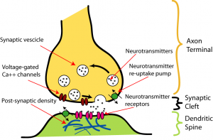
A synapse occurs between two neurons: a presynaptic neuron and a postsynaptic neuron. You can think of the presynaptic neuron as the sender and the postsynaptic neuron as the receiver. Below are major parts to a synapse:
- Axon terminal: An end of the presynaptic neuron’s axon. The axon terminal stores neurotransmitter in small capsules called vesicles.
- Synaptic cleft: The synaptic cleft is a gap between the presynaptic and postsynaptic neuron, which can become flooded with neurotransmitter.
- Dendritic spine: A small protrusion from the postsynaptic dendrite, which meets the presynaptic axon. Dendritic spines are plastic — dynamically changing shape and size, appearing and disappearing. It is believed spines are an integral part of learning and memory.
- Receptors: Proteins to which neurotransmitter binds. Receptors can open ion channels, possibly exciting the postsynaptic neuron.
Keep in mind, neurons don’t just interface with each other axon $\rightarrow$ dendrite. Synapses can also appear between axons and cell bodies, axons and axons, axons and axon terminals, etc. However, in these other interfaces, there are no dendritic spines.
Neurotransmitters & Receptors
Neurotransmitters are substances which are released by presynaptic neurons and cause changes in the postsynaptic neuron. The most direct way neurotransmitters affect the postsynaptic neuron is by either raising or lowing its membrane potential. Excitation and inhibition is surprisingly organized in the brain. These are not absolute rules, but hold generally:
- Neurotransmitter types are either excitatory or inhibitory, e.g. if a transmitter $s$ excites neurons, it never inhibits — no matter the receptor.
- Synapses are either excitatory or inhibitory, i.e. they release either an inhibitory or excitatory neurotransmitter but not both.
- Neurons are either excitatory or inhibitory, i.e. they release either inhibitory or excitatory neurotransmitters but not both.
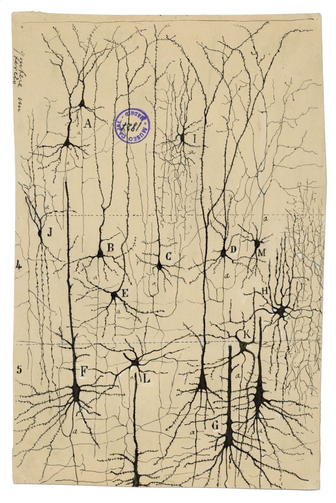
- In pyramidal neurons, like the ones drawn below, excitatory synapses (occasionally referred to as Type I) typically occur at the dendrites whereas inhibitory synapses (occasionally referred to as Type II) typically occur near or on the cell body.
There is a long list of neurotransmitters, but, in this post we look at the 2 most prevalent:
- Glutamate: binds to receptors which excite the postsynaptic neuron; accounts for 90% of all synaptic connections.
- GABA: binds to receptors which inhibit the postsynaptic neuron.
There are two categories of receptors found on postsynaptic neurons:
- Ionotropic: these are ion channels which are open when neurotransmitter binds to them.
- Metabotropic: these activate G-protein pathways (intracellular signaling mechanism) which can among other things, can indirectly open ion channels.
There can be multiple types receptors for a neurotransmitter. We’ll consider 2 glutamate receptors:
- AMPA: A quick-to-activate, fast-to-deactivate excitatory ionotropic receptor. Gates sodium and calcium.
- NMDA: A slow-to-activate, slow-to-deactivate excitatory ionotropic receptor. Gates sodium and calcium.
We’ll also consider 2 GABA receptors:
- GABA$_A$: A quick-to-activate, fast-to-deactivate iinhibitory onotropic receptor.
- GABA$_B$: A slow-to-activate, slow-to-deactivate inhibitory metabotropic receptor. G-proteins act as second messengers to open ion channels.
| Fast | Slow | |
|---|---|---|
| Excitatory | AMPA | NMDA |
| Inhibitory | GABA$_A$ | GABA$_B$ |
Physiology of Chemical Synapses
Synaptic transmission is a mechanism which allows one neuron to communicate with another: the presynaptic neuron neuron fires an action potential and releases transmitter, which opens the postsynaptic neuron’s ion channels. Looking closer at this three part act:
- Release: The presynaptic neuron fires an action potential. When the action potential reaches the axon terminal, membrane depolarization triggers voltage gated calcium channels to open. When the calcium enters the terminal, it causes vesicles to fuse to the terminal and dump their contents into the synaptic cleft.
- Activation: Transmitter crosses the synaptic clef and binds to receptors on the postsynaptic neuron. This causes the receptors to activate, opening ion channels and activating various chemical pathways.
- Deactivation: Postsynaptic channels become deactivated because (1) the concentration of neurotransmitter in the synaptic clef decreases, either by breaking down, or being reuptaken by the presynaptic neuron, and (2) transmitter releases from receptors.
A result of synaptic transmission is a PSP — a postsynaptic potential, i.e. a change in the postsynaptic neuron’s membrane potential at the site of the synapse. This change in potential helps excite or inhibit the postsynaptic neuron. For more about action potentials and neural excitability, you can read the previous part of this series.
Primer: Exponential Decay
The mathematical foundation for synaptic dynamics is largely based on exponential decay.
Exponential decay is the name for a process where the rate of decay of some quantity is proportional to the current value of that quantity, or:
$$\frac{dN}{dt} = -\lambda N$$
where $-\lambda$ is the decay rate and $N$ is the quantity. By integrating, we can find a closed form solution:
$$N(t) = N_0e^{-\lambda t}$$
where $N_0$ is the initial quantity and $N(t)$ is the quantity at time $t$.
In our case, the quantity is either directly or indirectly a measure of the number of ions in some part of the synapse, e.g. the fraction of active receptors which is dependent on the concentration in the synaptic cleft.
As a matter of convention, in neuroscience and other fields, it is often more popular to express exponential decays with $\tau$, referred to as the exponential time constant:
$$\tau = \frac{1}{\lambda}$$
so,
$$\frac{dN}{dt} = -\frac{N}{\tau}$$
and therefore,
$$N(t) = N_0e^{-\frac{t}{\tau}}$$
It turns out $\tau$ has some nice properties: when $t=\tau$, $N$ is $1/e$ its initial value. This happens to be the mean of the decay function. In other words: if we were modeling the fraction of open ion channels, $\tau$ would be the average time an ion channel spent open.
Play around with exponential decay, $\tau$, and half-life here:
We can also flip the direction of exponential decay:
$$\frac{dN}{dt} = N_{\infty} – \frac{N}{\tau}$$
where $N_{\infty}$ is the value N decays to. Or:
$$N(t) = N_{\infty} – N_{\infty}e^{-\frac{t}{\tau}}$$
Synaptic Dynamics
Synaptic Current
Aside from NMDA, which involves voltage gating dynamics, postsynaptic current can be modeled as:
$$I=\bar{g}_{s}P(V-E_{s})$$
where
- $V$ is the postsynaptic membrane potential
- $E_{s}$ is the Nernst potential.
- $\bar{g_s}$ is the maximum postsynaptic conductance, i.e. max permeability of the receptors.
- $P \in [0,1]$ is the probability a channel is open.
This equation should look familiar if you’ve read part I. Fundamentally, all this equation describes is how ions move across the postsynaptic neuron’s membrane through the ion channels controlled by synapse $s$ — the details merely say how. $V- E_s$ defines what direction ions are moving; $\bar{g_s}$ defines the max flow of ions across the membrane; and $P$ defines the open/closed dynamics of the channel — $P$ is what the rest of this discussion is about.
Just like a synapse, $P$ has presynaptic and postsynaptic components:
$$P=P_sP_{rel}$$
Where
- $P_s$ is the conditional probability a receptor activates given transmitter release occurs.
- $P_{rel}$ is the probability of neurotransmitter release.
For now, lets just assume $P_{rel}$ is always 1. Until we touch short term plasticity, all we will care about is $P_s$.
| $\tau$ | $E_{x}$ | |
|---|---|---|
| AMPA | ~5(ms) | ~0(mV) |
| NMDA | ~150(ms) | ~0(mV) |
| GABA$_A$ | ~6(ms) | ~-70(mV) |
| GABA$_B$ | ~150(ms) | ~-90(mV) |
Synaptic Conductance
$P_s$ can be modeled by a pair of transition rates, $\alpha_s$ and $\beta_s$, between an open and closed states.
$$\frac{dP_s}{dt} = \overbrace{\alpha_sT(t)(1 – P_s)}^{\text{rise}} – \overbrace{\beta_sP_s}^{\text{fall}}$$
$T(t)$ represents whether neurotransmitter is present in the synaptic clef. For simplicity, this just a square pulse. When neurotransmitter is present the receptor activates — fast enough that we can largely ignore deactivation (which I do in the visualization). When neurotransmitter is not present the open dynamics, $\alpha_s$ is 0.
You’ll notice that this can be rewritten to look like a pair of exponential decays, which you are familiar with!
$$\frac{dP_s}{dt} = \overbrace{\frac{1}{\tau_{rise}}T(t)(1 – P_s)}^{\text{rise}} – \overbrace{\frac{1}{\tau_{fall}}P_s}^{\text{fall}}$$
For receptors like AMPA, GABA$_A$, and GABA$_B$ the rise of P_s is rapid enough to treat it as instantaneous. Therefore we can simplify this as:
$$\frac{dP_s}{dt} = -\frac{P_s}{\tau_s}$$
or, after a presynaptic action potential
$$P_s \leftarrow 1$$
Hands on demo
…but first an overview of how these plots work.
Below you’ll find a few interactive plots to play around with various receptors.
These plots are my own concoction, so let me explain how they work:
The top left plot (vertices & edges) graphically represents the topology of a network of neurons. One vertex can represent multiple neuron. If you see a ring emanate from a vertex, the neuron(s) represented by that vertex fired.
The top right window lets you play around with some network parameters, i.e. properties of synapses or properties of neurons.
The bottom left plot shows the membrane potential of neuron $0$.
The bottom right plot shows the synaptic conductance from neuron $1 \rightarrow 0$
AMPA
When an AMPA receptor is activated, it raises the postsynaptic membrane potential; its effects are short, on the order of milliseconds.
Click on neuron ![]() to cause an EPSP.
to cause an EPSP.
NMDA
When an NMDA receptor is activated, it raises the postsynaptic membrane potential; its effects are long, on the order of hundreds of milliseconds. Unlike the other receptor types discussed in this post, NMDA receptors are voltage gated, meaning that even if NMDA is activated, ions do not necessarily flow. Rather, there must be other coincidental excitatory postsynaptic potentials from AMPA. In that way, NMDA receptors are coincidence detectors. The strong currents NMDA induces are believed to be an important mechanism in learning.
$$I = \bar{g}_{NMDA}G_{NMDA}P(V – 0)$$
where
$$G_{NMDA} = $$
Click on neuron ![]() to cause EPSPs.
to cause EPSPs.
GABA$_A$
When a GABA$_A$ receptor is activated, it lowers the postsynaptic membrane potential; its effects are short, on the order of milliseconds.
Click on neuron ![]() to cause an IPSP.
to cause an IPSP.
GABA$_B$
When a GABA$_B$ receptor is activated, it lowers the postsynaptic membrane potential; its effects are short, on the order of hundreds of milliseconds.
Click on neuron ![]() to cause an IPSP.
to cause an IPSP.
Release Probability and Short-Term Plasticity
The transmitter release probability $P_{rel}$ of synapses is dependent on the recent history of activation. In some cases, recent activity causes $P_{rel}$ to increase, in other cases it causes $P_{rel}$ to decrease, however, during quiet periods of inactivity, $P_{rel}$ returns to a neutral state. This process can be referred to as short-term plasticity (STP). When the history of activity causes a synapse to become temporarily stronger, we call it short-term facilitation (STF) and, inversely, when the history of activity causes a synapse to become temporarily weaker, we call it short-term depression (STD).
To model, short-term facilitation, it makes sense to have the $P_{rel}$ decay to a stable state $P_0$ but inch toward a either 0 or 1 after a presynaptic spike. We achieve this with the following equation:
$$\frac{dP_{rel}}{dt} = \frac{P_0 – P_{rel}}{\tau_P}$$
where $P_{rel} \rightarrow P_{rel} f_F(1 – P_{rel})$ when the presynaptic neuron fires.
In short-term depression, $P_{rel} \rightarrow P_{rel}f_D$ when the presynaptic neuron fires.
Short-term plasticity has some very interesting computational properties. Namely, synapses can perform high/low pass filtering. A high frequency input, under STF, becomes stronger, whereas a low frequency input is relatively weaker. Inversely, a high frequency input, under STD, becomes weaker, whereas a high frequency input is relatively stronger!
Learning & Memory
Hebbian Learning & Spike-timing dependent plasticity
There are many types of learning. Here we will touch on Hebbian learning. Hebbian learning postulates that
“When an axon of cell A is near enough to excite B and repeatedly or persistently takes part in firing it, some growth process or metabolic change takes place in one or both cells such that A’s efficiency, as one of the cells firing B, is increased” – Donald Hebb
or neurons that fire together wire together.
$$\frac{dw_i}{dt} = \eta v u_i$$
where $\eta$ is a learning rate, $v$ is the the postsynaptic neural response and $u_i$ is the presynaptic neural response. If both pre- and post-synaptic neurons fire together they are strengthened, if neither fire together they are not strengthened. Now, while there are problems with this original formulation, e.g. synapses only get stronger, it captures the gist of a common type of synaptic modification.
Spike-timing dependent plasticity (STDP) is a form of Hebbian learning which resolves some of the problems encountered with earlier models, namely it allows synapses to strengthen and weaken and it inherently involves competition between synapses all while avoiding the assumption of global, intracellular mechanisms. The intuition behind this rule is as follows: if a presynaptic neuron fires before a postsynaptic neuron does, it helped cause it to fire; if the presynaptic neuron fires after a postsynaptic neuron does, it did not cause it to fire; synapses learn the causal relationship between neurons.
This model works as follows:
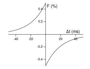
each time either the presynaptic or postsynaptic neuron fires, the synapse is updated according to some amount based on the difference in spike timing:
$$F(\Delta t) = \bigg\{\begin{array}{lr} A_+e^{\frac{\Delta t}{\tau_+}}, & \Delta t < 0 \\ -A_-e^{\frac{\Delta t}{\tau_-}}, & \Delta t > 0 \end{array}$$
STDP has several fascinating computational properties:
- Spike correlations: spikes between pre- and post-synaptic neurons become correlated through reinforcement.
- network latency: STDP can reduce network latency by reinforcing presynaptic neurons which consistently fire prior to the postsynaptic neuron.
- regulation: STDP regulates network firing rates, achieving a homeostatic effect , despite being quite stable at the local level.
Here is a javascript implementation of STDP taken from [1] — I’ve added a moving scatter plot, so you can see how the network weights evolve over time.
If you wait long enough (unfortunately quite a while), the distribution should look something like this:

Concluding Thoughts
In this post, we briefly viewed an important computational ingredient in the brain — synapses. We saw how they can pass signals between neurons and how they can regulate networks and filter information. We also briefly introduced Hebbian learning theory with STDP.
Lastly, a mind-boggling figure: it is estimated the average human brain has 0.15 quadrillion synapses [6], with around 7000 synapses per neuron in neocortex (probably a hotly debated number…). Usually, I think most figures of large numbers are kind of pointless — but, in this case, each member is dynamic and can represent information about the world. The mechanisms of the brain are rich and complex.
References
- Song, Sen, Kenneth D. Miller, and Larry F. Abbott. “Competitive Hebbian learning through spike-timing-dependent synaptic plasticity.” Nature neuroscience 3.9 (2000): 919.
- http://www.johndmurray.org/materials/teaching/tutorial_synapse.pdf
- http://www.ee.columbia.edu/~aurel/nature%20insight04/synaptic%20computation04.pdf
- http://www.scholarpedia.org/article/Spike-timing_dependent_plasticity#Basic_STDP_Model
- www.scholarpedia.org/article/Short-term_synaptic_plasticity
- Pakkenberg, Bente, et al. “Aging and the human neocortex.” Experimental gerontology 38.1-2 (2003): 95-99.
As someone with a biological background wanting to understand neuroscience from a computational perspective, this is an awesome resource! Can’t wait for the next post
Hey, I’m following your blog post (its been super informative so far!!) and I’m confused when it comes to implementing STDP. You mention that STDP modifies weights based on when spikes arrive, so its a function of time. When I’m coding this, do I have to keep a list of all the spikes that neuron A sends to neuron B and apply STDP on all of these spikes? Or do I only use the most recent spike that occurred and have the rest not modify the weight of the synapse at all? If you have any code samples for STDP, it would be great if you can share, there seems to be almost nothing I can find online for spiking neurons other than the math.
Cool post! Does the graph of exponential decay has its axis labelled the other way round? Should it be N versus tau?