Neurons are cells — small bodies of mostly water, ions, amino acids and proteins with remarkable electrochemical properties. They are the primary functional units of the brain. Our mental experiences — our perceptions, memories, and thoughts — are the result of the ebb and flow of salts across neural bi-lipid membranes and the synaptic transmissions between neurons. Understanding neurons and neural computation can help illuminate how our rich mental experiences are constructed and represented, the underlying principles of our behavior and decision making, as well as provide biological inspiration for new ways to process information and for artificial intelligence.

In this post, I give an interactive overview of ways to model neurons. This post is by no means intended to be comprehensive. Nothing new is being said here either. However, I hope it gives the curious reader an intuition about model neurons. The figure below lets you play with different models and their parameters. Don’t worry if you don’t know what a dynamical system is, what a bifurcation is, or even what an action potential is: those are briefly explained in the rest of this post.

Primer: Biology of the Neuron

Before we dive into mathematical models, we should first take a brief tour of the biology of a neuron, it all its glory (you can definitely skip this if you’ve taken any Neuroscience course).

Anatomy of a Neuron

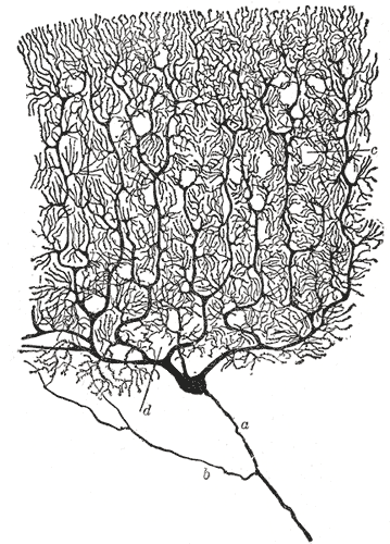
The first thing to appreciate about neurons is their specialized morphology, i.e. their form and structure. It allows them to receive information from thousands of other cells and communicate rapidly over large distances — up to a meter from the spinal cord to the feet!

 

Neurons receive signals from other neurons through synapses located – not exclusively – on their dendritic tree, which is a complex, branching, sprawling structure. If you are wondering what the king of dendritic complexity is, that would be the Purkinje cell, which may receive up to 100,000 other connections. Dendrites are studded with dendritic spines – little bumps where other neurons make contact with the dendrite.

Signals from the dendrites propagate to and converge at the soma – the cell’s body where nucleus and other typical cell organelles live.

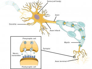
Coming off the soma is the axon hillock which turns into the axon. The axon meets other neurons at synapses. It allows a neuron to communicate rapidly over long distances without losing signal integrity. To allow signals to travel rapidly, the axon is myelinated – it is covered with interspersed insulators which allows the neuron’s signal to jump between insulated sections. To allow the signal to maintain integrity, the neuron signal in the axon is ‘all-or-nothing’ – it is a rather bit-like impulse, which we will discuss next.

Physiology of a Neuron

The second thing to appreciate about neurons is their specialized physiology — that is the cellular functions of neurons. The most striking feature of neural cellular function is the action potential. This is the mechanism which allows neurons to transmit information reliably over long distances without the transmission attenuating.

It is important to remember that neurons bathe in an extracellular solution of mostly water, salts and proteins. The forces caused by the movement of salts into and out of the cell and the different concentrations of these salts is the physical basis of the neuron’s remarkable behavior. There are sodium-potassium pumps which move sodium out of the cell and potassium in, so that the concentration of sodium outside the cell is higher than inside and the concentration of potassium outside the cell is lower then inside.

An action potential is a discrete event in which the membrane potential rapidly rises (depolarizes) and then falls (polarizes). This discrete event is all-or-nothing, meaning that if an action potential occurs at one part of the neurons membrane, it will also occur in the neighboring part, and so on until it reaches the axon terminal. Action potentials do not tend to travel backwards, because, once a section of the membrane has fired an action potential, electrochemical-forces hyper-polarize the region of membrane while the channels which were previously open close and become inactive for some duration of time.

 

The action potential is the result of different species of ions traveling across the cell membrane through channels and the activation and inactivation of those channels on different time scales. A stereotypical action potential occurs as follows:

1. Equilibrium: The neuron’s equilibrium membrane potential is near -70 mV — roughly the Nernst Equilibrium of $E_{K^+}\approx-75$. At equilibrium the, net current is 0 — inward and outward currents are balanced.
2. Depolarization: Incoming excitatory signals depolarize the membrane. Quick-to-respond voltage gated $Na^+$ channels are activated, and $Na^+$ rushes in, pushing the membrane potential higher. Slower-to-respond $K^+$ channels open, and $K^+$ rushes out, pushing the membrane potential lower.
3. Amplification: If the neuron becomes more stimulated or is stimulated rapidly, many more $Na^+$ channels are activated than $K^+$ channels. This causes a feedback loop where the influx of $Na^+$ causes more $Na^+$ channels to activate.
4. Repolarization: Eventually the membrane potential is near the Nernst Equilibrium of $Na+$ as the sodium channels are maximally open. The slower $K^+$ channels catch up to $Na^+$, which repolarizes the membrane potential. Meanwhile, the $Na+$ channels become inactive.
5. Hyper-polarization: $K^+$ channels are open while $Na^+$ channels are inactive, causing the membrane potential to dip below its typical equilibrium point, near the $K^+$ Nernst equilibrium.
6. Refractory Period: The $Na^+$ channels, take a while to become deinactivated, meaning after an action potential, they remain incapable of opening again for a period of time. The period in which most $Na^+$ channels is called the absolute refractory period (the neuron cannot spike no matter the strength of the stimulus) while the period in which many $Na^+$ channels are inactivated is called the relative refractory period (the neuron can spike given a sufficiently strong stimulus).

As we will see below, some models — the Hodgkin-Huxley model in particular — capture the essence of an action potential well. With these theoretical models, you can explore the computational properties of action potentials and other interesting neural phenomena.

Spike Trains

Spike trains are the language of neurons. People tend to think of spikes as point-events and spike trains as point-processe. We describe these with the neural response function:

$$\rho(t) = \sum\limits^{k}_{i=1}\delta(t – t_i)$$

where an impulse is defined as the dirac delta function (which is convenient for counting things):

 

$$\delta(t) =
\begin{cases}
1& \text{ if t = 0},\\
0 & otherwise
\end{cases}
$$

Often, it is useful for analysis to assume spike trains are generated by random processes. Assuming spikes are independent of each other, we can model this point process is a Poisson process, in which we know the probability $n$ spikes occur in the interval $\Delta T$:

$$P\{n \text{ spikes occur in } \Delta t\}=\frac{(rt)^n}{n!}exp(-rt)$$

To generate spikes according to a Poisson point process, generate a random number $r$ in a sufficiently small time interval, such that only 1 spike should occur, and check whether $r < firing Rate \Delta t$. However, make sure that $firing Rate \Delta t < 1$.

 

Primer: Dynamical Systems

Bifurcations & Dynamical Systems

Many model neurons are dynamical systems — that is they describe the state of the neuron as some vector which evolves over time according to some equations. Each point in the space of the model has a corresponding gradient, or direction in which it will evolve. Many things about a model can be inferred just by looking at its phase portrait. There are two example phase portraits below. These portraits are visually dense — this section will attempt to explain how to understand them.

Equilibria

Dynamical systems are at equilibum when they do not change with time. More formally, $x$ is an equilibrium point of system $x’=f(x)$ if $f(x)=0$. There are only 5 kinds of fixed points in dynamical systems we will consider.

• stable nodes attract all points within a neighborhood. Stable nodes occur when all eigenvalues are negative and real.
• unstable nodes repel all points within a neighborhood. Unstable nodes occur when all eignevalues are positive and real.
• stable foci attract all points within a neighborhood by spiraling inward. Stable foci occur when eigenvalues are complex conjugate with negative real parts.
• unstable foci repel all points within a neighborhood by spiraling outward. Unstable foci occur when eigenvalues are complex conjugate with positive real parts.
• saddles attract along two directions and repel along two directions. Saddles occur when eigenvalues are real with opposite sign.

Null-clines

A two dimensional neuron model, like the ones above, has two null-clines — that is two lines along which one of the partial derivatives is 0. By crossing one of the null-clines, the evolution of one of the variables changes direction. A great deal about a dynamical system can be ascertained just by looking at its null-clines, including the location of the fixed points.

Bifurcations

Bifucations are the qualitative change in a dynamical system — a qualitative change is the appearance or disappearance of an equilibrium point or limit cycle. These changes occur when one parameter changes — this is the so called, bifurcation parameter. In neuron models, the bifurcation parameter is often the input current, $I$. There are only four kinds of bifurcations we will consider:

• saddle node bifurcation: At a saddle node bifurcation, a stable node and unstable node annihilate each other after merging into a saddle node. In a neuron model, prior to a saddle node bifurcation is the disappearance of a stable equilibrium.
• saddle node bifurcation on a limit cycle: Similar to a saddle node bifurcation, however, the bifurcation point occurs on a limit cycle. This latter detail is important, since at the equilibrium point, the limit cycle has infinite period, allowing the periodicity to change continuously with the bifurcation parameter. When the saddle node does not occur on a limit cycle, the periodicity is discontinuous. This has implications for the computational properties of neurons.
• Super-critical Andronov-Hopf bifurcation: At a super-critical Andronov-Hopf bifurcation, a stable equilibrium transitions to an unstable equilibrium as a limit cycle emerges and grows. Near a super-critical Andronov-Hopf bifurcation, a neuron can spike if its input is rhythmic.
• Sub-critical Andronov-Hopf bifurcation: At a sub-critical Andronov-Hopf bifurcation, an unstable equilibrium transitions to a stable equilibrium as a limit cycle shrinks and then disappears.

Okay, now lets dive in!

Models

Hodgkin-Huxley Model Neuron

The Hodgkin Huxley model neuron is a remarkable feat of physiological modeling, which earned Alan Hodgkin and Andrew Huxley the 1963 Nobel Prize in Physiology or Medicine. It is an important model in computational neuroscience. Interestingly, this model was constructed by studying the squid giant axon, which controls squids’ water jet propulsion reflex – its large diameter allows for easy experimentation.

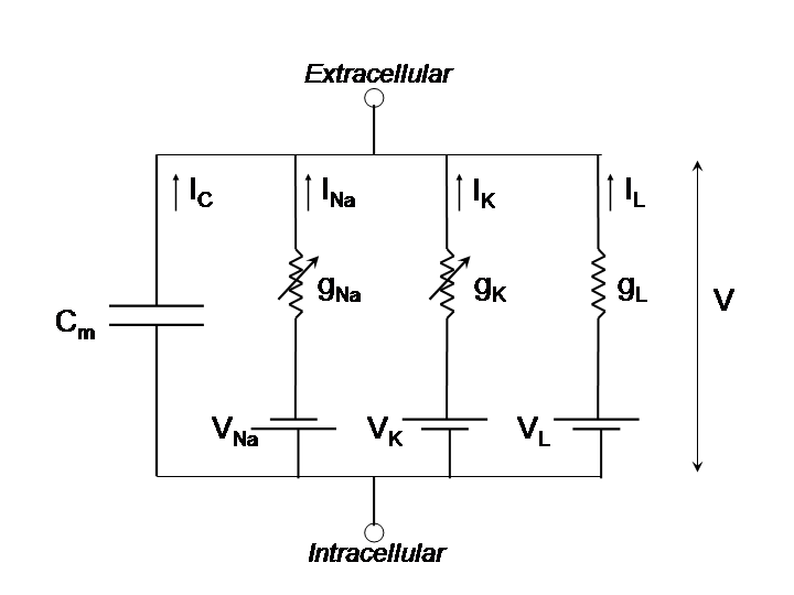
As you will see, there is a lot of math, but, essentially, the Hodgkin-Huxley model describes the dynamics of a neuron as a circuit with currents which are activated, and inactivated at different timescales and at different voltages.

The model includes three currents, $I_{Na}$, $I_{K}$, and $I_{leak}$ which influence the membrane potential. $I_{leak}$ is not gated, rather $Cl^-$ ions slowly leak across the membrane. $I_{K}$ is gated by $n$, a unitless variable $[0,1]$, which represents the activation of $K^+$voltage gated channels (increasing the flow of potassium). $I_{Na}$ current is gated by $m$ as well as $h$, were $m$ is a unitless variable $[0, 1]$ (increasing the flow of sodium), which represents the activation of $Na^+$ voltage gated channels and where $h$ is a unitless variable $[0, 1]$ which represents the inactivation of $Na^+$ channels (stopping flow of sodium).

$$\begin{align}C\dot{V} &= \overbrace{-g_L(V-E_L)}^{I_{leak}} – \overbrace{g_{Na}m^3h(V – E)}^{I_{Na}} – \overbrace{g_Kn(V-E_K)}^{I_K} \\ \dot{n} &= \frac{n_{\infty}(V) – n}{\tau_n(V)} \\\dot{m} &= \frac{m_{\infty}(V) – m}{\tau_m(V)} \\ \dot{h} &= \frac{h_{\infty}(V) – h}{\tau_h(V)} \end{align}$$

where

$$\begin{align} n_{\infty} &= \frac{\alpha_n}{\alpha_n + \beta_n}, &\tau_n &=\frac{1}{\alpha_n + \beta_n} \\ m_{\infty} &= \frac{\alpha_m}{\alpha_m + \beta_m}, &\tau_m &=\frac{1}{\alpha_m + \beta_m} \\ h_{\infty} &= \frac{\alpha_h}{\alpha_h + \beta_h}, &\tau_h &=\frac{1}{\alpha_h + \beta_h} \end{align}$$

where

$$\begin{align} \alpha_n(V) &= 0.01\frac{10 – V}{exp(\frac{10 – V}{10}) – 1}, &\beta_n(V) &= 0.125exp(\frac{-V}{80}) \\ \alpha_m(V) &= 0.1\frac{25 – V}{exp(\frac{25 – V}{10}) – 1}, &\beta_m(V) &= 4exp(\frac{-V}{18}) \\ \alpha_h(V) &= 0.07exp(\frac{- V}{20}), &\beta_h(V) &= \frac{-V}{exp(\frac{30 – V}{10}) + 1} \end{align}$$

$\alpha_x$ models the rate at which gate $x$ transitions to being open  while $\beta_x$ models the rate at which gate $x$ transitions to being closed.

The Hodgkin-Huxley model is the most accepted model. It is also the most complex model we will consider in this post. The following models are more abstract and will lack some features of the Hodgkin-Huxley model, however they are more easy to analyze and simulate.

Artificial Neurons

Artificial Neurons – those used in artificial neural networks – are a beautiful reduction of biology. They are an abstraction of neural behavior which reduces the behavior into a few key features: (a) they integrate (sum together) signals over all incoming synapses, (b) they transform the integral signal according to a non-linear function:

We can write (a) formally as:

$$\begin{equation}I_i = \sum\limits_{j}w_{ij}v_j\end{equation}$$

Where neuron $j$ is the pre-synaptic neuron, $i$ is the post-synaptic neuron, $v_j$ is the signal from $j$ to $i$ and $w_{ij}$ is the strength of the synapse.

and (b) formally as:

$$v_i=f(I_i)$$

where $f(I_i)$ is typically a sigmoid or linear rectifier function.

Pretty simple, but a little hokey. These are better called units rather than neurons, since they don’t spike. Nonetheless, the output from these units can be interpreted as the a firing rate. Despite their simplicity, these units are useful for exploring aspects of neural computation. Not only that but they are used in state-of-the-art AI algorithms. It has been shown that artificial neural networks with just one hidden layer are capable of approximating any function.

The strength of these kind of neurons stem from being differentiable — even when stacked in networks. This property minimize or maximize some goal to learn an arbitrary function. However, due to their simplicity, e.g. the lack of a spiking mechanism and persistent state and their simplicity, they aren’t realistic models of the biology.

Integrate & Fire

The integrate and fire model is a widely used model, typically in exploring the behavior of networks. This simple model captures several features of neural behavior: (a) a membrane threshold after which the neuron spikes and resets, (b) a refractory period during which the neuron cannot fire, and (c) a state — this is a dynamical system in which the membrane potential, the state, evolves over time.

$$\frac{dv}{dt}\tau m=-v(t) + RI(t)$$

$$v \leftarrow v_{reset} \text{  if  } v >= v_{threshold}$$

This model lacks a true mechanism for spike generation, however. In stead we merely draw a vertical line when the neuron spikes. Furthermore, the membrane threshold and refractory period are absolute, whereas in real neurons, they can change depending on the state of the neuron. These neurons are also incapable of resonating. This is not to say this model is not useful — the integrate and fire neuron has the most basic features of a spiking neuron and it is very easy to reason about. It has been used in many interesting explorations of network behavior.

Conductance Based Models

Conductance based models are sets of equations like the Hodgkin Huxley model — they represent neurons with (1) the conductances of various ion channels and (2) the capacitance of the cell membrane. Conductance based models are a simple but varied class of models. Unlike the integrate and fire model, conductance based models are capable of generating spikes. Some are also capable of resonating, oscillating, rebound spiking, bi-stability spiking, and so on.

 

 

The current flowing across the neuron membrane is described by these models as follows:

$$I = C\dot{V} + I_{Na} + I_{Ca} + I_{K} + I_{Cl}$$

(Kirchhoffs law)

The dynamics of the models are archtypically describe as the following:

$$C_m\frac{dV}{dt} = \sum\limits_{i}g_i(V_i – V) + I_{external}$$

$$g_i = g_i$$

As there are many ways to skin a cat, there are many ways to make a model spike. We have already looked at the Hodgkin Huxley model above, but since it is a 4 dimensional system, it does not yield to analysis easily. Below, let’s look at a one dimensional system and a two dimensional system which are based on the dynamics of sodium channels and sodium & potassium channels respectively.

$I_{Na,p}$

The persistent sodium or $I_{Na,p}$ model has only a sodium channel and this sodium channel responds instantly to the current membrane potential, which, due to the relatively rapid dynamics of sodium channels, is not a bad idea. This lets us have a very simple, one dimensional model. Now, if we recall the physiology of the action potential, the lack of a potassium channel suggests that the dynamics of the model should be incapable of reseting itself, and indeed we add a condition to manually reset the neuron after a spike.

$$\begin{align}C\dot{V} &= \overbrace{-g_L(V-E_L)}^{\text{leak}} – \overbrace{g_{Na}m_{\infty}(V)(V – E)}^{\text{instantaneous }I_{Na,p}} \\ m_{\infty}(V)&=\frac{1}{(1 + exp\{\frac{V_{1/2} – V}{k}\})}\end{align}$$

Looking at the state space, below a certain input current, there are two fixed points, one of which corresponds to the membrane potential at equilibrium. The other corresponds to a peak membrane potential of the spike. Separating the two is, of course, a source point.

Spiking occurs after the model undergoes a bifurcation: the equilibrium fixed point and the source annihilate each other causing the neuron to tend toward spiking, no matter its initial state.

$I_{Na,p} + I_{K}$

The persistent sodium plus potassium or $I_{Na,p}+I_{K}$ model adds potassium channels to the  $I_{Na,p}$ model. This potassium channel, unlike the sodium channel, does not activate instantaneously, rather it activates as we would expect it to: slower than $Na$. Unlike $I_{Na, p}$ this model is two dimensional.

$$\begin{align}C\dot{V} &= \overbrace{-g_L(V-E_L)}^{\text{leak}} – \overbrace{g_{Na}m_{\infty}(V)(V – E)}^{\text{instantaneous }I_{Na,p}} – \overbrace{g_Kn(V-E_K)}^{I_K} \\ m_{\infty}(V)&=\frac{1}{(1 + exp\{\frac{V_{1/2} – V}{k}\})} \\ \dot{n} &= \frac{n_{\infty}(V) – n}{\tau(V)}\end{align}$$

A common way to model conductance based models is to treat an entire neuron as a single compartment — that is, to ignore all the structural complexity of the dendrites. Signals originating in dendritic branches propagate and coalesce in complex ways, which is typically very computationally expensive to model. While conductance based models are more realistic than the others we have seen above, you should be aware of this draw back. To account for these features, one would use the cable equation.

Simple Dynamical Models

If you weren’t constrained to thinking about ion channels — that is, if, for a moment, you could allow yourself to look past the wetware, the biological hardware — could you capture aspects of cell behavior relevant to neural computation while maintaining the simplicity needed for tractable analysis and simulation. The intuition behind Eugene Izhikevich’s simple model is that a good model needs 1) a fast variable describing the membrane potential and 2) a slow variable describing the recovery dynamics. The recovery variable does not need to explicitly represent a particular ionic current, rather it can describe the sum of all recovery currents. The simple model is constructed in such a way that by tweaking its parameters correctly, it can be near a saddle node bifurcation or an Andronof-Hopf bifurcation. This has great benefits when simulating networks of neurons. Not only is the computational cost reduced by simplifying the dynamics to 2 variables described by relatively simple equations, one model can be used to represent a multitude of neural properties.

$$\begin{align}\frac{dv}{dt} &= 0.04v^2 + 5v + 140 – u + I \\ \frac{du}{dt} &= a(bv – u)\end{align}$$

$$\text{if } v \ge v_{peak} \text{, then }  \begin{cases}
v &\leftarrow c,\\
u &\leftarrow u + d
\end{cases}$$

Computational Properties of Neurons

Neurons decode information from other neurons, transform this information, and then encode information to other neurons in the form of spikes. The computational properties of neurons enable them to perform this operation. Below are some examples of computational properties (the list is by no means comprehensive).

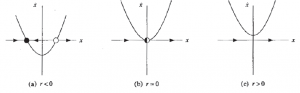
Class 1, 2, and 3 Neurons

One way to look at the computational powers of neurons is to look at their F-I functions — that is, their gain functions. Hodgkin proposed 3 classes of neurons based on this metric, which are represented in the below figures:

 

 

However, this classes can be described richer with dynamical systems. In class 1 behavior is the result of saddle node bifurcations on a limit cycle, whereas class 2 behavior is the result of the other 3 kinds of bifurcations. Class 3 behavior can occur when a fixed point suddenly moves (faster than the membrane potential can) such that the neuron spikes, and then returns to the shifted equilibrium state.

It should be said that there are many other ‘types’ of neurons. That is, there is more to neurons than their gain functions. In fact there is a project at the Allen Institute working on the lumping of neurons into types. They have an amazing open source brain cell database.

Integrators & Resonators

We can also consider whether neurons are either integrators or resonators, which, from a dynamical systems point of view, whether neurons undergo saddle node bifurcations or Andronof-Hopf bifurcations.

Integrators accumulate signals until their membrane potential reaches a well defined threshold (a separatrix defining a basin of attraction). Closely timed signals are added together and have greater affect than when far apart. Integrators are coincidence detectors. Some integrators are type 1 neurons.

 

Resonators resontate (oscillate) in response to incoming signals. Resonators do not necessarily have clearly defined thresholds. In the case of models near a super-critical Andronof-Hopf bifurcation, some spiral trajectories lead outside the basin of attraction but others do not. The threshold is fuzzy.  Unlike integrators, resonators are most sensitive to a narrow band of frequencies. Resonators are coincidence detectors as well, but they are also frequency detectors. All resonators are type 2 neurons.

Concluding Thoughts

The way neurons process information is fascinating, complex, and there are still many things we do not know (which any passionate scientist should find exciting). The models discussed in this post are far from perfect. These models do not account for important aspects of neurons such as the complex structure of their dendritic trees or local field potentials (though such models do exist). However, keeping in mind that we will likely fall short of capturing all relevant aspects of the brain relevant for cognition for some time, simulation is a very practical and interesting way to study neural computation. I hope this series of posts can inspire tinkerers, hackers, and programmers to play with such models and possible discover something new.

References

• Eugene M. Izhikevich (2007) Equilibrium. Scholarpedia, 2(10):2014.
• Yuri A. Kuznetsov (2006) Andronov-Hopf bifurcation. Scholarpedia, 1(10):1858.
• Yuri A. Kuznetsov (2006) Saddle-node bifurcation. Scholarpedia, 1(10):1859.
• Izhikevich, Eugene M. Dynamical systems in neuroscience. MIT press, 2007.
• Dayan, Peter, and Laurence F. Abbott. Theoretical neuroscience. Vol. 806. Cambridge, MA: MIT Press, 2001.